Literature Review

The problem of detecting fake news has a strong corollary with other types of spam detection, such as online review spam detection. Jindal and Liu (2008) divided Amazon spam comments into three classes: bogus reviews—spam intended to praise/defame the product in order to raise/lower its status within the store; reviews on brands, where the text praises/defames the brand/company behind the product with no information regarding product-specific experience; finally, non-reviews, including advertisements, questions/answers, and random texts (i.e. the comment has no sentiment, real or fake). Classification was performed using logistic regression for each task. A first-pass screening of duplicate comments can be eliminating comments with a certain level of similarity; in the case of text data, one can use the Jaccard similarity, which takes the set of all words in comments \(d_{i},d_{j}\) and calculates \(J_{i,j} =\frac{\mathrm{unique \enspace words}(d_{i}) \cap \mathrm{unique \enspace words}(d_{j})}{\mathrm{unique \enspace words}(d_{i}) \cup \mathrm{unique \enspace words}(d_{i})}\). In their analysis of these reviews, they found that 90% of reviewers on a subset of products had a maximum comment Jaccard similarity (vs. any reviewer) of 0.1, with the fewest having a Jaccard similarity of around 0.5, with the number slowly increasing up to a maximum score of 1, with 6% of reviewers having a maximum Jaccard score of 1. Users may either be spam accounts or genuine accounts accidentally sending duplicate reviews. In the context of fake news headlines, Jaccard similarity can be used as a distance metric in a k-nearest neighbors classifier, though this simple implementation may have bias towards classifying certain news topics or sources with certain styles (e.g. tabloids) as fake news. Brand reviews and non-reviews are the easier classification problems, as bogus reviews have a level of verisimilitude. The features used for classifying the former two types of spam include review-centric features, reviewer features, and product features, with textual features being particularly of interest. Frequency of positive and negative words in reviews, and frequency of brand name mentions, numbers, capital letters, and all-capital words were examined. Additionally, cosine similarity between reviews and product features was specifically helpful in detecting advertisements, with cosine similarity \(S_{\cos}(d_{i},d_{j})=\frac{d_{i} \dot d_{j}}{||d_{i}|| \enspace ||d_{j}||}\), with \(d_{i}\) being an \(1 \times n, n=\mathrm{\# \enspace unique \enspace words \enspace in \enspace dataset}\) feature vector with each entry being the count of a unique word; since large values of \(S_{\cos}\) indicate high degrees of similarity in overlap of vocabulary, \(1-S_{\cos}(d_{i},d_{j})\) can be also used as a distance metric for classification tasks. An \(L_{1}\) version using Manhattan distance or \(L_{p}\) using \(p\)-dimensional Minkowski distance can be formulated by replacing the \(L_{2}\) distance metric with the \(L_{p}\)-norm. For classification of bogus reviews, the task involved looking at reviewer history to examine biases in reviews of similar products using outliers: positive reviews on poorly-reviewed products, negative reviews on well-reviewed products, and polarized reviews on products with average ratings. Jindal and Liu (2008) applied uplift modeling, a technique often found in marketing contexts, to assess likelihood of classification as spam based on four different types of reviewers: positive and negative reviewers (those \(\pm 1 \sigma\)) in terms of sentiment, and positive and negative same-brand reviewers. Uplift per decile was implemented to compare the likelihood of positive spam classification to these four classes compared to random chance. A summary of uplift modeling and uplift per decile can be found in Gutierrez and Gérardy (2017), though the methods in this paper does not have random assignment of treatments so causality is not relevant. Reviewers who repeatedly gave negative reviews for the same brand were most likely across all deciles to be classified as spam, whereas those with positive reviews generally were less likely than random to be classified as spam.

Horne and Adali (2017) proposed a method of classification using features based on complexity, style, and intended psychological effect by using various NLP toolkits for Python, and applied an ANOVA to explore their datasets. Real news article titles are more likely on average to contain fewer proper nouns than fake or satire news article titles, while real news article bodies were more likely to contain positive words and less likely to contain negative words than fake news articles. Their Linear SVM was applied to a dataset of 75 real articles, 75 fake news articles, and 75 satire articles, with performance assessed on the mean of 5-fold cross-validation of one-versus-one classification tasks. The SVM performed best on distinguishing satire article bodies from real article bodies, and performed worst on distinguishing satire article titles from fake news article titles.

One common method of dimensionality reduction of text datasets is the term-frequency inverse-document-frequency (\(tfidf(D,d,t)=tf(t,d) \times idf(t,D)\)) where \(D\) is the set of all data, \(d \in D\), and \(t\) are the set of terms within all documents \(D\). The term frequency within a document can be described by the raw count divided by the total number of terms in the document \(tf(t,d)=\frac{f_{t,d}}{\sum_{t' \in d} f_{t',d}}\), or through alternative measures of \(tf(t,d)\) such as the raw count, binary, or through a normalization method such as log normalization \(tf(t,d)=\log(1+f_{t,d})\) or through double normalization with strength \(K\), \(tf(t,d)=K+(1-K)\frac{f_{t,d}}{\max_{\{t' \in d\}} f_{t',d}}\). Inverse document frequency \(idf(t,D)\) is a measure that increases with the rarity of a term, and is classically measured by \(idf(t,D)=\log \frac{|D|}{|d \in D: t \in d|}\) where \(|D|\) is the number of documents and \(|d \in D: t \in d|\) is the number of documents where \(t\) can be found. Alternatives includes the smooth IDF \(1 + \log \frac{|D|}{1+|d \in D: t \in d|}\) which reduces the deweighting of common document-wide terms (e.g. ‘for,’ ‘the,’ ‘and’) and the probabilistic IDF \(\log \frac{|D|-|d \in D: t \in d|}{|d \in D: t \in d|}\) which further deweights the most common document-wide terms. TFIDF is implemented in feature extraction tasks for "Ahmed et al. (2018) and Ahmed, Traore, and Saad (2017).

Ahmed, Traore, and Saad (2017) preprocessed the data by removing unnecessary characters, tokenizing the resulting words, removing stop words—common words such as pronouns, prepositions, and infinitives, and stemming—reducing conjugated forms e.g. '{run, runner, running, drink, drinker, drinking} \(\rightarrow\) '{run, run, run, drink, drink, drink}. From these, \(n\)-grams (word sequences of length \(n\)) were extracted, and the top \(k\) \(n\)-grams were selected for each sample. For the top 50,000 cleaned \(n=1\)-grams (i.e. single words), the accuracy of the linear SVM was 92.0%.

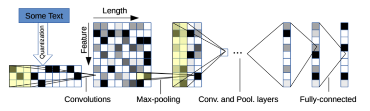
Figure 3: Character-level convolution

Zhang, Zhao, and LeCun (2016) proposed a character-level method of classification of text using 1-dimensional convolutional neural networks, allowing for flexibility with and generalization to problems with different character sets (e.g. Greek alphabet, Hangul, Emoji). The proposed method works by assigning each character (including padding and unknown characters as specific entities) as unique integer IDs which are converted to one-hot vectors within the character embedding space. Each sample is now represented by a 2D array which can be thought of as a time series of one-hot vectors. From this point, the embdedded data is convolved using several filters and max-pooled several times before flattening to a series of fully-connected layers with dropout before the final output layer, which has 1 node in binary classification and regression problems and \(k\) nodes in a \(k\)-way classification problem.

The example model structure is offered in small or large configurations in the example. Within the convolutional stage, it uses 6 rounds of ReLu-activated 1-D convolution with feature sizes of either 256 (small) or 1024 (large); the first two 1-D convolutional layers have a filter size of 7 and are both followed by a max-pooling layer with a pooling number of 3. After this second max-pooling layer, the data passes through the 3 ReLu-activated 1-D convolutional layers with filter size of 3 before the final 1-D convolutional layer, which also has a filter size of 3 and is followed by another max-pooling layer with a pooling number of 3. This feature array is flattened as it gets passed to the two dropout-regulated fully-connected layers, which are either of size 1024 (small) or 2048 (large); the dropout probability for their experiments was set to \(p_{\mathrm{dropout}}=0.5\). In order to control for generalization error through data augmentation, on some experiments using the character-level CNN the authors implemented a weighted thesaurus method, where new samples are copied from existing samples, and the sentences are scanned for replaceable words (i.e. words with a synonym); the probability that \(n\) words are replaced in a given sample follows a geometric distribution where \(P(n=x) = (1-p)p^{x}, x\in \mathbb{Z} \geq 0, p \in (0,1)\); when it is decided that a word is replaced, it is replaced with a synonym with index \(s\) in the similarity-sorted list which also follows a geometric distribution, with the probability of choosing index \(s\) is \(P(s=y) = (1-q)q^{y}, y \in \mathbb{Z} \geq 0, q \in (0,1)\). This method is unfortunately agnostic to whether or not the replaced word(s) are load-bearing (i.e. their replacement by synonym(s) completely changes the meaning of a sentence). The authors set \(p=q=0.5\) for their analysis, though this provides an hyperparameter that can be further inspected. With the dataset from Ahmed, Traore, and Saad (2017) the concern of augmentation using the thesaurus method is that its random assignment of replacement words may directly affect the classification task because unusual patterns of speech are often found in spam, whereas this augmentation may be better fit for tasks such as sentiment analysis or topic/ontological classification. The character-level CNN was compared to to classical NLP methods such as bag-of-words and its TFIDF, bag-of-\(n\)-grams and its TFIDF, and bag-of-means on word embedding, as well as deep learning methods such as a long-short term memory (LSTM) network and word-based convolutional networks using word2vec or a lookup table.

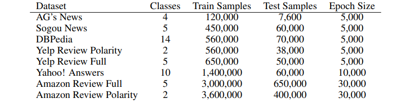
Figure 4: Comparison of classification tasks in Zhang, Zhao, and LeCun (2016). Epoch size is measured by dividing training size by batch size.

The authors’ models performed the best in tasks with large sample sizes (i.e. the latter four entries in []), with \(n\)-gram methods performing best for the tasks smaller datasets, indicating its quality for implementation in large datasets and potential commercial applications. From their results, the authors learned that the semantics of the task do not affect the classification capability of character-level CNN and that considering uppercase characters to be separate from their lowercase counterparts was not helpful for larger datasets; in environments and learning tasks where capitalization conveys less meaning, distinguishing between the two is likely to be not as important. In the case of fake news detection, it is possible that fake news headlines or body texts use nonstandard capitalization (e.g. Phrases In Title Case, PHRASES IN ALL CAPS) and thus whether uppercase letters should be retained in the embedding ought to be tested as part of this paper’s methodology.